Wildfire Regression & Resampling-based CI
Figure 10.40
Every notebook here is yours to modify — swap in your own colors, styling, and data, and use it as a starting point for your own publication-quality graphics.
OLS regression of California wildfire area over time (1987–2019), null-hypothesis shuffle test, and resampling-based confidence interval for the slope. This is the static view of the notebook — click below to run it live in your browser.
▶ Run interactively in browser ↗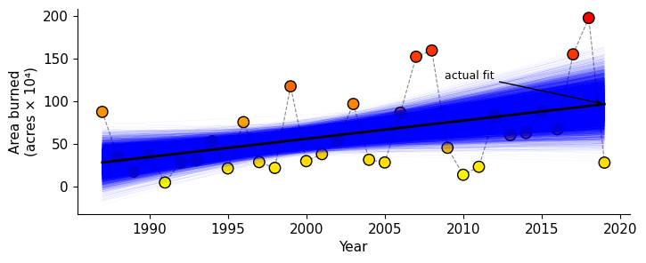
Figure 10.40 Resampling-based confidence interval: 10,000 resampled regression lines for California wildfire area over time.
Setup — imports & data
import numpy as np
import matplotlib.pyplot as plt
from scipy import stats
from plot_utils import plot_scatter, finish_plot, vline_labeled

# California wildfire data — ACRES_total (CAL FIRE data is publicly available at https://www.fire.ca.gov/our-impact/statistics
years = np.array([
    1987, 1988, 1989, 1990, 1991, 1992, 1993, 1994, 1995, 1996, 1997, 1998, 1999, 2000, 2001, 2002, 2003, 2004, 2005, 2006,
    2007, 2008, 2009, 2010, 2011, 2012, 2013, 2014, 2015, 2016, 2017, 2018, 2019
])
acres = np.array([
     873000,  345000,  173400,  365200,   44200,  282745,  309779, 526219,  209815,  752372,  283885,  215412, 1172850,  295026,
     377340,  538216,  965770,  311024,  279214,  863345, 1520362, 1593690,  451969,  134462,  228599,  829224,  601635,  625540,
     880899,  669534, 1548429, 1975086,  277285
])
xi = np.array([years.min(), years.max()])
OLS regression
slope_obs, intercept, r, p, se = stats.linregress(years, acres)
print(f"Slope: {slope_obs/1e4:.2f} x10^4 acres/year  |  R^2: {r**2:.3f}  |  p: {p:.4f}")

fig, ax = plt.subplots(figsize=(8, 3))
plot_scatter(ax, years, acres)

ols_y  = (slope_obs * xi + intercept) / 1e4
null_y = np.mean(acres) / 1e4
ax.plot(xi, ols_y,      color='blue', lw=2.5, zorder=3)
ax.plot(xi, [null_y]*2, color='red',  lw=2.5, zorder=3)

ax.set_xlim(years.min() - 1, years.max() + 3)
ax.text(years.max() + 0.4, ols_y[1], f'm = {slope_obs/1e4:.2f}',
        color='blue', fontweight='bold', va='center', fontsize=10)
ax.text(years.max() + 0.4, null_y, 'm = 0',
        color='red',  fontweight='bold', va='center', fontsize=10)
finish_plot(ax, 'Year', 'Area burned\n(acres x 10^4)')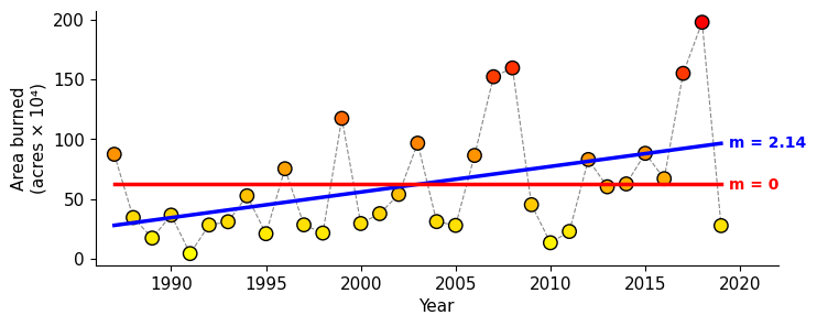
NHST — 10,000 shuffled regression lines
np.random.seed(0)
N = 10_000

shuffle_slopes, shuffle_intercepts = np.array([
    stats.linregress(years, np.random.permutation(acres))[:2] for _ in range(N)
]).T

fig, ax = plt.subplots(figsize=(8, 3))
plot_scatter(ax, years, acres)
for s, b in zip(shuffle_slopes, shuffle_intercepts):
    ax.plot(xi, (s * xi + b)/1e4, color='red', lw=0.1, alpha=0.1)
ax.plot(xi, (slope_obs * xi + intercept)/1e4, color='blue', lw=2.5, zorder=4)
finish_plot(ax, 'Year', 'Area burned\n(acres x 10^4)')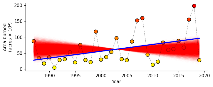
n_right = int(np.sum(shuffle_slopes >=  slope_obs))
n_left  = int(np.sum(shuffle_slopes <= -slope_obs))
p_perm  = (n_right + n_left) / N
print(f"Two-sided permutation p-value: {p_perm:.4f}  ({n_left} left + {n_right} right)")

counts, _ = np.histogram(shuffle_slopes / 1e4, bins=50)
m = slope_obs / 1e4

fig, ax = plt.subplots(figsize=(6, 2))
ax.hist(shuffle_slopes / 1e4, bins=50, color='red', edgecolor='white', linewidth=0.5)
vline_labeled(ax,  m, 'm')
vline_labeled(ax, -m, '-m', ls='--')
ax.text(-m - 0.15, counts.max() * 0.65, f'{n_left} simulations\nwith m_i <= -m', ha='right', va='top')
ax.text( m + 0.15, counts.max() * 0.65, f'{n_right} simulations\nwith m_i >= m',  ha='left',  va='top')
ax.set_xlim(-m * 3, m * 3)
finish_plot(ax, 'Slope', 'Count')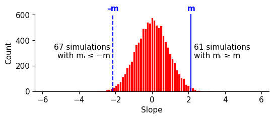
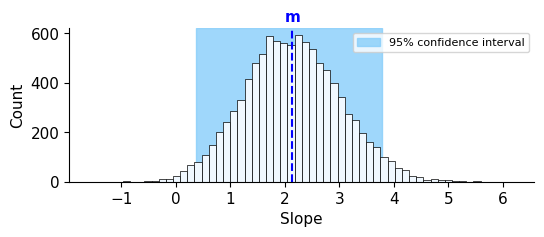
Resampling-based CI — 10,000 resampled regression lines
np.random.seed(42)
n = len(years)

boot_slopes, boot_intercepts = np.array([
    stats.linregress(years[idx], acres[idx])[:2]
    for idx in (np.random.randint(0, n, n) for _ in range(N))
]).T

fig, ax = plt.subplots(figsize=(8, 3))
plot_scatter(ax, years, acres)
for s, b in zip(boot_slopes, boot_intercepts):
    ax.plot(xi, (s * xi + b)/1e4, color='blue', lw=0.1, alpha=0.2)
ax.plot(xi, (slope_obs * xi + intercept)/1e4, color='black', lw=2, zorder=4)
ax.annotate('actual fit',
    xy=(xi[1], (slope_obs * xi[1] + intercept)/1e4),
    xytext=(xi[1] - 7, (slope_obs * xi[1] + intercept)/1e4 + 30),
    arrowprops=dict(arrowstyle='->', color='black', lw=1),
    fontsize=9, ha='right')
finish_plot(ax, 'Year', 'Area burned\n(acres x 10^4)')
ci_low = 2 * slope_obs - np.percentile(boot_slopes, 97.5)
ci_high = 2 * slope_obs - np.percentile(boot_slopes, 2.5)
print(f"95% pivotal resampling-based CI: [{ci_low/1e4:.2f}, {ci_high/1e4:.2f}] x10^4 acres/year")
x_lo, x_hi = boot_slopes.min() / 1e4, boot_slopes.max() / 1e4
fig, ax = plt.subplots(figsize=(6, 2))
ax.axvspan(ci_low/1e4, ci_high/1e4, alpha=0.8, color='lightskyblue',
label='95% confidence interval', zorder=0)
ax.hist(boot_slopes / 1e4, bins=50, facecolor='aliceblue', edgecolor='black',
linewidth=0.5, zorder=1)
vline_labeled(ax, slope_obs / 1e4, 'm', ls='--')
ax.set_xlim(x_lo - (x_hi - x_lo) * 0.15, x_hi + (x_hi - x_lo) * 0.15)
ax.legend(loc='upper right', fontsize=8, framealpha=0.8)
finish_plot(ax, 'Slope', 'Count')