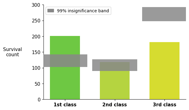
Titanic Survival by Class
Figures 8.37, 8.40, 8.41
Every notebook here is yours to modify — swap in your own colors, styling, and data, and use it as a starting point for your own publication-quality graphics.
Observed and expected contingency tables, NHST null distribution, and Mt. Fuji insignificance-band plot for survival by passenger class. This is the static view of the notebook — click below to run it live in your browser.
▶ Run interactively in browser ↗
Note: This notebook uses
plot_utils — a helper module bundled in the interactive environment.
Setup — imports, data & NHST simulation
import numpy as np
import matplotlib.pyplot as plt
import matplotlib.patches as mpatches
from matplotlib.patches import Rectangle, FancyBboxPatch
from matplotlib.collections import PatchCollection
from plot_utils import despine

# Colors
ROW_COLORS = ['#6EC843', '#B5D440', '#D6DC30']   # green, yellow-green, yellow
NO_COLOR   = '#F5923E'                            # orange — did not survive
BLUE_DARK  = '#29A9E1'
BLUE_LIGHT = '#A8D8EA'

# Observed counts  [Yes=survived, No=did not survive]
o = np.array([[201, 123],   # 1st class
              [118, 166],   # 2nd class
              [181, 528]])  # 3rd class

n          = int(np.sum(o))
row_totals = np.sum(o, axis=1).astype(int)   # [324, 284, 709]
col_totals = np.sum(o, axis=0).astype(int)   # [500, 817]

# Expected counts under independence
e = np.array([col_totals / n * r for r in row_totals])

# Chi statistic: sum of |O - E| / E
def chi_stat(obs, exp):
    return np.sum(np.abs(obs - exp) / exp)

chi_obs = chi_stat(o, e)

# Shuffle resampling (null distribution)
pool = np.array([1]*col_totals[0] + [0]*col_totals[1])
n1, n2, n3 = [int(x) for x in row_totals]

np.random.seed(0)
N = 10_000
sim_counts = np.empty((N, 3, 2), dtype=int)
sim_chi    = np.empty(N)

for i in range(N):
    s = pool.copy()
    np.random.shuffle(s)
    c1, c2, c3 = s[:n1], s[n1:n1+n2], s[n1+n2:]
    sim_counts[i] = [[c1.sum(), n1 - c1.sum()],
                     [c2.sum(), n2 - c2.sum()],
                     [c3.sum(), n3 - c3.sum()]]
    sim_chi[i] = chi_stat(sim_counts[i], e)

n_extreme = int(np.sum(sim_chi >= chi_obs))
p_str = '< 0.0001' if n_extreme == 0 else f'= {n_extreme / N:.4f}'
print(f'X_obs = {chi_obs:.4f}')
print(f'Simulations with X_i >= X_obs: {n_extreme}  (p {p_str})')
print(f'Expected counts (rounded):\n{np.round(e, 1)}')
Figure 8.37 — Observed contingency table
fig, ax = plt.subplots(figsize=(4.8, 2.6))
ax.axis('off')

cell_text = [
    ['1st class', str(o[0, 0]), str(o[0, 1]), str(row_totals[0])],
    ['2nd class', str(o[1, 0]), str(o[1, 1]), str(row_totals[1])],
    ['3rd class', str(o[2, 0]), str(o[2, 1]), str(row_totals[2])],
    ['',          str(col_totals[0]), str(col_totals[1]), str(n)],
]
cell_colors = [
    [ROW_COLORS[0], ROW_COLORS[0], NO_COLOR, 'white'],
    [ROW_COLORS[1], ROW_COLORS[1], NO_COLOR, 'white'],
    [ROW_COLORS[2], ROW_COLORS[2], NO_COLOR, 'white'],
    ['white', 'white', 'white', 'white'],
]

tbl = ax.table(
    cellText=cell_text,
    colLabels=['', 'Yes', 'No', ''],
    cellColours=cell_colors,
    colWidths=[0.35, 0.20, 0.20, 0.25],
    loc='center',
    cellLoc='center',
    bbox=[0.02, 0.02, 0.96, 0.82]
)
tbl.auto_set_font_size(False)
tbl.set_fontsize(12)

for (r, c), cell in tbl.get_celld().items():
    cell.set_edgecolor('white')
    cell.set_linewidth(3)
    if r == 0:
        cell.set_facecolor('none')
        if c in [0, 3]:
            cell.set_visible(False)
    if r == 4:
        cell.set_facecolor('white')
        cell.set_edgecolor('none')
    if c == 3 and r < 4:
        cell.set_facecolor('white')
        cell.set_edgecolor('none')
    if c == 0 and 0 < r < 4:
        cell.set_text_props(fontweight='bold')

ax.text(0.57, 0.98, 'survived?', ha='center', va='top',
        fontsize=13, fontweight='bold', transform=ax.transAxes)

plt.tight_layout()
plt.show()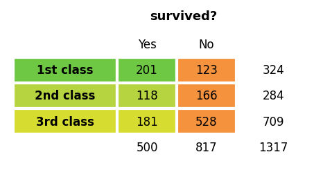
Expected counts under independence
fig, ax = plt.subplots(figsize=(3.6, 2.6))
ax.axis('off')

e_rounded   = np.round(e, 1)
cell_text   = [[f'{e_rounded[i, 0]}', f'{e_rounded[i, 1]}'] for i in range(3)]
cell_colors = [[BLUE_LIGHT, BLUE_LIGHT] for _ in range(3)]

tbl = ax.table(
    cellText=cell_text,
    rowLabels=['1st class', '2nd class', '3rd class'],
    colLabels=['Yes', 'No'],
    cellColours=cell_colors,
    rowColours=[BLUE_LIGHT] * 3,
    loc='center',
    cellLoc='center',
    bbox=[0.22, 0.02, 0.65, 0.62]
)
tbl.auto_set_font_size(False)
tbl.set_fontsize(12)
for (r, c), cell in tbl.get_celld().items():
    cell.set_edgecolor('white')
    cell.set_linewidth(3)
    if r == 0:
        cell.set_facecolor(BLUE_DARK)
        cell.set_text_props(color='white', fontweight='bold')
    if c == -1 and r > 0:
        cell.set_facecolor(BLUE_LIGHT)
        cell.set_text_props(fontweight='bold')

ax.text(0.55, 0.85, 'expected (E)', ha='center', va='top',
        fontsize=13, fontweight='bold', color=BLUE_DARK, transform=ax.transAxes)
ax.text(0.55, 0.75, 'survived?', ha='center', va='top',
        fontsize=11, fontweight='bold', transform=ax.transAxes)
plt.tight_layout()
plt.show()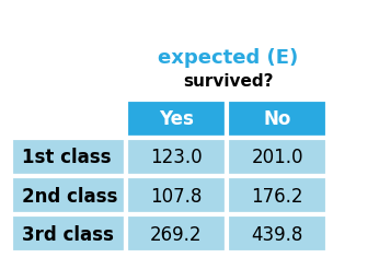
Figure 8.40 — NHST null distribution
fig, ax = plt.subplots(figsize=(10, 2.5))

ax.hist(sim_chi, bins=31, color='lightpink', alpha=0.6, edgecolor='black')
ax.axvline(chi_obs, color='black', lw=1.5)

ax.text(chi_obs, 1.02, r'$X_{obs}$', ha='center', va='bottom',
        transform=ax.get_xaxis_transform(), fontsize=12)

ax.text(chi_obs + 0.02, 0.92,
        f'{n_extreme} simulations\nwith $X_i \geq X_{{obs}}$\n\np {p_str}',
        va='top', ha='left', transform=ax.get_xaxis_transform())

ax.text(0.02, 1, 'null distribution', va='top', ha='left',
        transform=ax.transAxes)

ax.set_xlabel('X-value')
ax.set_ylabel('Count', rotation=0, ha='center', va='center', labelpad=25)
ax.set_xlim(0, 2)
ax.set_ylim(0, 1000)
despine(ax)
plt.show()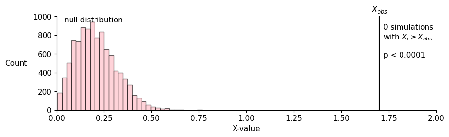
Figure 8.41 — Mt. Fuji: survived counts with 99% insignificance band
fig, ax = plt.subplots(figsize=(6, 4))

x       = np.arange(3)
xlabels = ['1st class', '2nd class', '3rd class']
pct     = 1   # 99% band (0.5th - 99.5th percentile)

# Colored bars (observed survived counts)
ax.bar(x, o[:, 0], color=ROW_COLORS, width=0.6, zorder=3)

# Gray 99% insignificance bands
bands = [
    Rectangle(
        (xi - 0.45, np.percentile(sim_counts[:, i, 0], pct / 2)),
        0.9,
        np.percentile(sim_counts[:, i, 0], 100 - pct / 2)
        - np.percentile(sim_counts[:, i, 0], pct / 2)
    )
    for i, xi in enumerate(x)
]
pc = PatchCollection(bands, facecolor='#888888', edgecolor='none', alpha=0.85, zorder=4)
ax.add_collection(pc)

ax.set_xticks(x)
ax.set_xticklabels(xlabels, fontweight='bold')
ax.set_ylim(0, 300)
ax.set_ylabel('Survival\ncount', rotation=0, ha='center', va='center', labelpad=45)

gray_patch = mpatches.Patch(color='#888888', label='99% insignificance band')
ax.legend(handles=[gray_patch], loc='upper left', frameon=True,
          fontsize=10, handlelength=1.5)

despine(ax)
plt.show()