T-Cell Count: Three-Group Comparison
Figures 7.20, 7.23–7.24
Every notebook here is yours to modify — swap in your own colors, styling, and data, and use it as a starting point for your own publication-quality graphics.
Omnibus resampling test and pairwise post-hoc comparisons — with p-values and 99% confidence intervals — for T-cell counts across three groups: a control (A) and two drugs (B, C). This is the static view of the notebook — click below to run it live in your browser.
▶ Run interactively in browser ↗Setup — imports & data
%matplotlib inline
import numpy as np
import matplotlib.pyplot as plt
import seaborn as sns
from matplotlib.patches import FancyBboxPatch
from plot_utils import despine, MAD

grpA = np.array([0.28, 0.34, 0.37, 0.47, 0.47, 0.58, 0.63, 0.76, 0.47, 0.51, 0.59,
                 0.61, 0.66, 0.76, 0.7 , 0.79, 0.83, 0.71, 0.92, 0.88, 1.01, 1.02,
                 0.77, 1.08, 1.05, 1.07, 1.47, 1.2 , 1.28, 1.33, 1.43, 1.36, 1.45,
                 1.49, 1.56, 1.68, 1.84, 1.86, 1.95, 2.04, 2.23, 2.2 , 2.22, 2.3 ,
                 2.44, 2.41, 2.56, 2.64, 2.67, 2.85, 2.93, 2.64, 2.74, 3.87, 4.86])
grpB = np.array([0.27,  0.5 ,  0.59,  0.78,  0.94,  0.97,  1.11,  1.08,  1.84,
                  1.72,  1.6 ,  1.53,  1.61,  1.67,  1.84,  2.22,  2.09,  2.17,
                  2.31,  2.99,  2.77,  2.74,  2.81,  2.99,  3.04,  3.17,  3.36,
                  3.54,  3.76,  3.97,  3.86,  3.92,  4.29,  4.54,  4.59,  4.66,
                  4.86,  5.53,  5.5 ,  5.8 ,  5.76,  5.9 ,  6.01,  6.12,  6.63,
                  6.88,  7.07,  7.5 ,  7.97,  8.33,  8.69,  8.77,  9.  ,  9.15,
                  9.91, 10.3 , 12.68, 14.28])
grpC = np.array([round(0.4 * a + 0.5 * b, 1) for a, b in zip(grpA, grpB)])

COLOR_A = '#2c99e3'  # blue   -- Control (A)
COLOR_B = '#e6484f'  # red    -- Drug 1 (B)
COLOR_C = '#2ca866'  # green  -- Drug 2 (C)

groups = {'A': grpA, 'B': grpB, 'C': grpC}
colors = {'A': COLOR_A, 'B': COLOR_B, 'C': COLOR_C}

for name, g in groups.items():
    print(f"{name}: n={len(g):>3}  median={np.median(g):.2f}  var={np.var(g):.2f}")
The data
fig, ax = plt.subplots(figsize=(5, 5))
sns.swarmplot(data=[grpA, grpB, grpC], ax=ax, size=6,
              palette=[COLOR_A, COLOR_B, COLOR_C])
ax.set_xticks([0, 1, 2]); ax.set_xticklabels(['A', 'B', 'C'])
ax.set_ylabel('T-cell count')
despine(ax)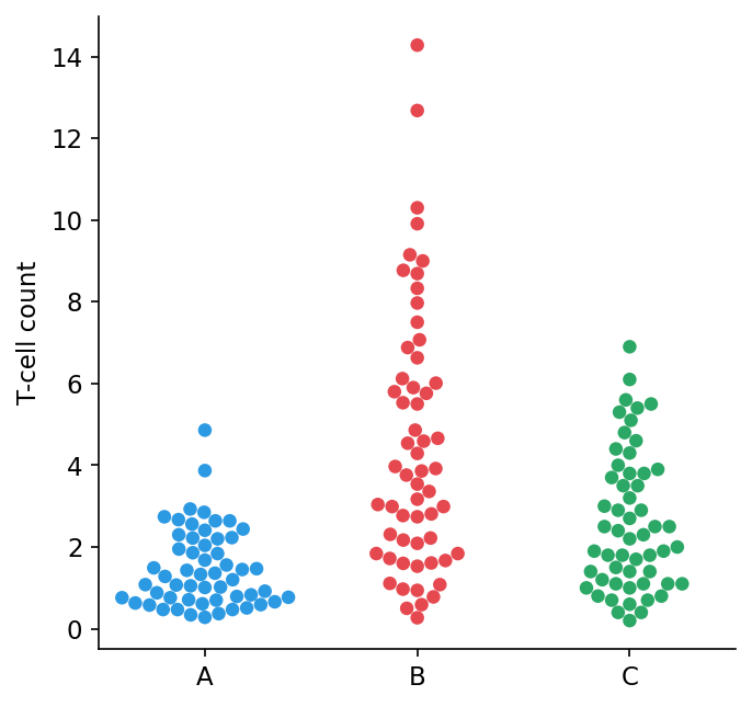
Figure 7.20 — Omnibus test
def f_statistic(groups):
    grand_median = np.median(np.concatenate(groups))
    between = sum(len(g) * abs(np.median(g) - grand_median) for g in groups)
    within  = sum(np.sum(np.abs(g - np.median(g))) for g in groups)
    return between / within


def resample_F(groups, n=10_000, seed=0):
    demedianed = [g - np.median(g) for g in groups]
    np.random.seed(seed)
    resampled = [np.random.choice(g, size=(n, len(g)), replace=True) for g in demedianed]
    return np.array([f_statistic([r[i] for r in resampled]) for i in range(n)])

dataset = [grpA, grpB, grpC]
Fobs = f_statistic(dataset)
Fs = resample_F(dataset, seed=0)

n_extreme = int(np.sum(Fs >= Fobs))
p_omnibus = n_extreme / len(Fs)
print(f"F_obs = {Fobs:.2f}")
print(f"{n_extreme} of {len(Fs)} simulations had F >= F_obs  ->  p = {p_omnibus:.4f}")

fig, ax = plt.subplots(figsize=(9, 5))
ax.hist(Fs, bins=100, color='#f6d78b', edgecolor='none')
ax.set_xlim(0, 0.7)
ax.set_xlabel('F-value')
ax.set_ylabel('Count')
despine(ax)

ax.text(0.05, ax.get_ylim()[1] * 0.12, 'null distribution', fontweight='bold', fontsize=12)
ax.axvline(Fobs, color='black', lw=1.5)
ax.text(Fobs, 1.02, f'F$_{{obs}}$ = {Fobs:.2f}', ha='center', va='bottom',
        fontweight='bold', transform=ax.get_xaxis_transform())
ax.text(Fobs + 0.015, ax.get_ylim()[1] * 0.42,
        f'{n_extreme} simulations\nwith F $\\geq$ F$_{{obs}}$\np = {p_omnibus:.4f}',
        fontweight='bold', va='top')

# Inset: swarm plot of the raw T-cell counts by group, as a small "card" in the
# upper right (mirrors the textbook figure's rounded-box inset).
card = FancyBboxPatch((0.60, 0.50), 0.38, 0.46, transform=ax.transAxes,
                       boxstyle='round,pad=0.006,rounding_size=0.02',
                       linewidth=1, edgecolor='#dddddd', facecolor='white', zorder=3)
ax.add_patch(card)

axins = ax.inset_axes([0.635, 0.545, 0.31, 0.35])
axins.set_zorder(4)
sns.swarmplot(data=[grpA, grpB, grpC], ax=axins, size=2.5,
              palette=[COLOR_A, COLOR_B, COLOR_C])
axins.set_xticks([0, 1, 2]); axins.set_xticklabels(['A', 'B', 'C'], fontsize=9)
axins.set_ylabel('T-cell count', fontsize=9)
axins.tick_params(labelsize=8)
despine(axins)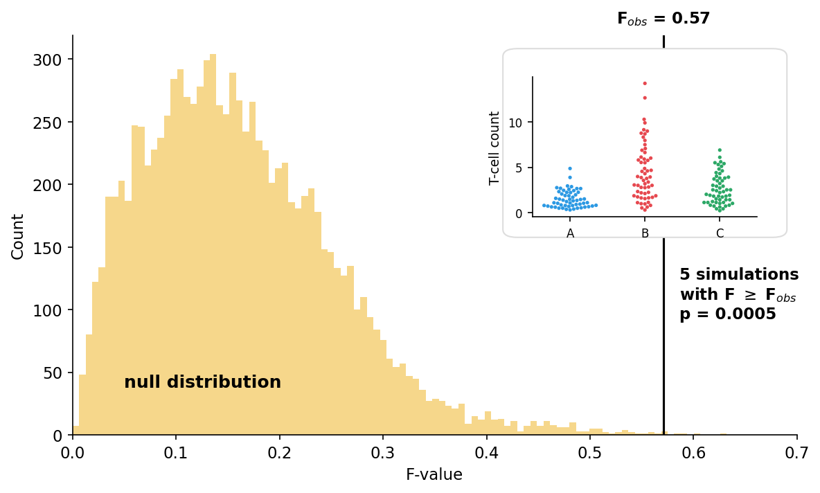
Figure 7.20 Omnibus test for the data set of T-cell counts in three groups (a control group and two drug groups).
Choosing big-box vs. two-box
def choose_method(A, B):
    vA, vB = np.var(A), np.var(B)
    return 'two-box' if (vA > 2 * vB or vB > 2 * vA) else 'big-box'


def pairwise_bootstrap(A, B, n=10_000, seed=0):
    """Two-sided resampling test for median(B) - median(A), using whichever of
    big-box / two-box the variance ratio calls for."""
    method = choose_method(A, B)
    dobs = np.median(B) - np.median(A)

    np.random.seed(seed)
    if method == 'two-box':
        Ad, Bd = A - np.median(A), B - np.median(B)
        rA = np.random.choice(Ad, (n, len(A)), replace=True)
        rB = np.random.choice(Bd, (n, len(B)), replace=True)
    else:
        pooled = np.concatenate([A, B])
        rA = np.random.choice(pooled, (n, len(A)), replace=True)
        rB = np.random.choice(pooled, (n, len(B)), replace=True)
    ds = np.median(rB, axis=1) - np.median(rA, axis=1)

    p = (np.sum(ds >= abs(dobs)) + np.sum(ds <= -abs(dobs))) / n
    return dobs, ds, p, method

for (n1, n2) in [('A', 'B'), ('A', 'C'), ('B', 'C')]:
    v1, v2 = np.var(groups[n1]), np.var(groups[n2])
    ratio = max(v1, v2) / min(v1, v2)
    print(f"{n1} vs {n2}: var ratio = {ratio:.2f}x  ->  {choose_method(groups[n1], groups[n2])}")
Figure 7.23 — Pairwise p-values
alpha = 0.01
pairs = [('A', 'B'), ('A', 'C'), ('B', 'C')]

fig, axs = plt.subplots(3, 2, figsize=(11, 9),
                         gridspec_kw={'width_ratios': [1, 3], 'hspace': 0.5})

for row, (n1, n2) in enumerate(pairs):
    A, B = groups[n1], groups[n2]
    dobs, ds, p, method = pairwise_bootstrap(A, B, seed=0)

    ax_sw, ax_hist = axs[row, 0], axs[row, 1]

    sns.swarmplot(data=[A, B], ax=ax_sw, size=3, palette=[colors[n1], colors[n2]])
    ax_sw.set_xticks([0, 1]); ax_sw.set_xticklabels([n1, n2])
    despine(ax_sw)

    # explicit range keeps bin edges (and so bar widths) identical across rows
    ax_hist.hist(ds, bins=30, range=(-3, 3), color='#e8e8e8', edgecolor='black', linewidth=0.7)
    ax_hist.set_xlim(-3, 3)
    ax_hist.set_ylim(top=ax_hist.get_ylim()[1] * 1.15)
    top = ax_hist.get_ylim()[1]

    # line stops short of the top, leaving room for the label above it
    line_top = top * 0.55
    ax_hist.vlines(dobs, 0, line_top, color='black', lw=1.3)
    ax_hist.vlines(-dobs, 0, line_top, color='black', lw=1.3, linestyle='--')

    # dobs can be negative, so figure out which line (solid or dashed) is on the right
    xlo, xhi = ax_hist.get_xlim()
    right_x, left_x = abs(dobs), -abs(dobs)
    if dobs >= 0:
        left_tag, right_tag = r'$-\Delta_{obs}$', f'$\\Delta_{{obs}}$ = {dobs:.2f}'
    else:
        left_tag, right_tag = f'$\\Delta_{{obs}}$ = {dobs:.2f}', r'$-\Delta_{obs}$'

    ax_hist.text(left_x, line_top + 0.08 * top, left_tag, ha='center', va='top', fontsize=9)

    n_extreme = int(np.sum(ds >= abs(dobs)) + np.sum(ds <= -abs(dobs)))
    p_label = 'p < 0.0001' if n_extreme == 0 else f'p ≈ {p:.4g}'
    stats_x = right_x + 0.02 * (xhi - xlo)
    ax_hist.text(right_x, line_top + 0.08 * top, right_tag,
                 ha='center', va='top', fontsize=9, fontweight='bold')
    ax_hist.text(stats_x, line_top + 0.00 * top, f'{n_extreme} simulations',
                 ha='left', va='top', fontsize=8.5)
    ax_hist.text(stats_x, line_top - 0.08 * top, r'more extreme than $\Delta_{obs}$',
                 ha='left', va='top', fontsize=8.5)
    ax_hist.text(stats_x, line_top - 0.16 * top, p_label,
                 ha='left', va='top', fontsize=8.5)

    ax_hist.set_ylabel('Count')
    if row == 2:
        ax_hist.set_xlabel(f'$\\tilde{{X}}_{{{n2}}} - \\tilde{{X}}_{{{n1}}}$')
    despine(ax_hist)

axs[0, 0].set_title('Pairwise comparisons', fontweight='bold', loc='left')
axs[0, 1].set_title('Null distribution with p-value', fontweight='bold', loc='left')
Figure 7.23 Pairwise comparisons for groups A, B and C, each yielding a p-value.
Figure 7.24 — Pairwise confidence intervals
def resample_medians(x, n=10_000):
    rs = np.random.choice(x, size=(n, len(x)), replace=True)
    return np.median(rs, axis=1)


def reflected_ci(dobs, d_resampled, alpha=0.01):
    lo = 2 * dobs - np.percentile(d_resampled, 100 * (1 - alpha / 2))
    hi = 2 * dobs - np.percentile(d_resampled, 100 * alpha / 2)
    return lo, hi

np.random.seed(1)
resampled_medians = {name: resample_medians(g) for name, g in groups.items()}

fig, axs = plt.subplots(3, 2, figsize=(11, 9),
                         gridspec_kw={'width_ratios': [1, 3], 'hspace': 0.5})

for row, (n1, n2) in enumerate(pairs):
    A, B = groups[n1], groups[n2]
    dobs = np.median(B) - np.median(A)
    d_resampled = resampled_medians[n2] - resampled_medians[n1]
    lo, hi = reflected_ci(dobs, d_resampled, alpha)

    ax_sw, ax_ci = axs[row, 0], axs[row, 1]

    sns.swarmplot(data=[A, B], ax=ax_sw, size=3, palette=[colors[n1], colors[n2]])
    ax_sw.set_xticks([0, 1]); ax_sw.set_xticklabels([n1, n2])
    despine(ax_sw)

    # shared bins/range keep bars comparable across rows
    ax_ci.hist(d_resampled, bins=20, range=(-5, 5), color='#c9e6c3', edgecolor='#6fae63', linewidth=0.7)
    ax_ci.set_xlim(-5, 5)
    ax_ci.set_ylim(top=ax_ci.get_ylim()[1] * 1.25)
    top = ax_ci.get_ylim()[1]
    xlo, xhi = ax_ci.get_xlim()

    # band capped below the bars so Delta_obs's line can rise above it
    ax_ci.axvspan(lo, hi, ymin=0, ymax=0.85, color='#a9cdf0', alpha=0.5, zorder=0)

    line_top = top * 0.9
    ax_ci.vlines(dobs, 0, line_top, color='black', lw=1.3)
    ax_ci.axvline(0, color='black', lw=1, linestyle='--')

    ax_ci.text(-0.015 * (xhi - xlo), top * 0.65, 'zero (null value)',
               rotation=90, rotation_mode='anchor', ha='right', va='center', fontsize=8.5)

    ax_ci.text(dobs, top * 0.99, r'$\Delta_{obs}$', ha='center', va='top', fontweight='bold')

    excludes_zero = not (lo <= 0 <= hi)
    mark = '✔' if excludes_zero else '✘'
    ax_ci.text(0.97, 0.6, f'{n1} vs {n2}\n{mark}', transform=ax_ci.transAxes,
               ha='right', va='top', fontweight='bold')

    ax_ci.set_ylabel('Count')
    if row == 2:
        ax_ci.set_xlabel('Group difference')
    despine(ax_ci)

axs[0, 0].set_title('Pairwise comparisons', fontweight='bold', loc='left')
axs[0, 1].set_title('Confidence intervals', fontweight='bold', loc='left')

# one legend for the whole figure, not per-row
fig.legend(handles=[
    plt.Rectangle((0, 0), 1, 1, fc='#c9e6c3', ec='#6fae63', label='resampling distribution'),
    plt.Rectangle((0, 0), 1, 1, fc='#a9cdf0', alpha=0.5, label='99% CI'),
], loc='upper right', bbox_to_anchor=(0.99, 0.99), frameon=False, fontsize=9)
Figure 7.24 Pairwise comparisons for groups A, B and C, each with a 99% confidence interval for the group difference.