Swimsuit vs Wetsuit Swimming Speed
Figures 6.37–6.43
Every notebook here is yours to modify — swap in your own colors, styling, and data, and use it as a starting point for your own publication-quality graphics.
Dot plots, paired-differences plot, and independent vs paired null distributions for paired swim speed data. This is the static view of the notebook — click below to run it live in your browser.
▶ Run interactively in browser ↗
Note: This notebook uses
plot_utils — a helper module bundled in the interactive environment.
Setup — imports, data & simulations
import numpy as np
import matplotlib.pyplot as plt
import seaborn as sns
from plot_utils import despine

COLOR_SWIM = '#E85420'   # orange — Swimsuit
COLOR_WET  = '#1040B5'   # blue   — Wetsuit

swimsuit = np.array([1.49, 1.37, 1.35, 1.27, 1.12, 1.64, 1.59, 1.52, 1.50, 1.45, 1.44, 1.41])
wetsuit  = np.array([1.57, 1.47, 1.42, 1.35, 1.22, 1.75, 1.64, 1.57, 1.56, 1.53, 1.49, 1.51])
deltas   = wetsuit - swimsuit
dobs     = np.mean(wetsuit) - np.mean(swimsuit)

BINS = np.arange(-0.225, 0.230, 0.005)

bigbox = np.concatenate([swimsuit, wetsuit])
np.random.seed(0)
N = 10_000
ds_sw  = np.mean(np.random.choice(bigbox, size=(N, len(swimsuit))), axis=1)
ds_wt  = np.mean(np.random.choice(bigbox, size=(N, len(wetsuit))),  axis=1)
ds_ind = ds_wt - ds_sw

np.random.seed(0)
signs   = np.random.choice([-1, 1], size=(N, len(deltas)), replace=True)
ds_pair = np.mean(deltas * signs, axis=1)

n_ind_lo  = int(np.sum(ds_ind  <= -dobs))
n_ind_hi  = int(np.sum(ds_ind  >=  dobs))
n_pair_lo = int(np.sum(ds_pair <= -dobs))
n_pair_hi = int(np.sum(ds_pair >=  dobs))
print(f'dobs = {dobs:.4f} m/s')
print(f'Independent: {n_ind_lo} <= -Delta_obs, {n_ind_hi} >= Delta_obs')
print(f'Paired:      {n_pair_lo} <= -Delta_obs, {n_pair_hi} >= Delta_obs')
Figure 6.37 — Dot plot with group means
fig, ax = plt.subplots(figsize=(5, 4.5))
sns.swarmplot(data=[swimsuit, wetsuit], ax=ax,
              palette=[COLOR_SWIM, COLOR_WET], size=8)
mean_s, mean_w = np.mean(swimsuit), np.mean(wetsuit)
ax.hlines(mean_s, -0.35, 0.35, colors='black', lw=2.5, zorder=5)
ax.hlines(mean_w,  0.65, 1.35, colors='black', lw=2.5, zorder=5)
ax.annotate('', xy=(0.5, mean_w), xytext=(0.5, mean_s),
            arrowprops=dict(arrowstyle='<->', color='black', lw=1.5,
                            mutation_scale=15))
ax.set_xticks([0, 1])
ax.set_xticklabels(['Swimsuit', 'Wetsuit'], fontweight='bold')
ax.set_ylim(1.08, 1.82)
ax.set_xlim(-0.55, 1.55)
ax.set_ylabel('Swimming speed\n(m/sec)', rotation=0, ha='center', va='center', labelpad=50)
despine(ax)
plt.tight_layout()
plt.show()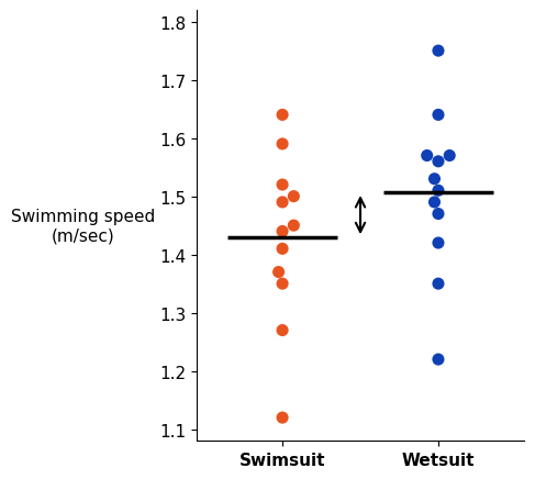
Figure 6.38 — Independent null distribution
fig, ax = plt.subplots(figsize=(8, 3))
ax.hist(ds_ind, bins=BINS, color='#c8c8c8')
ax.hist(ds_ind[np.abs(ds_ind) >= dobs], bins=BINS, color='black', edgecolor='black')
ax.axvline(-dobs, color='black', lw=1.5, linestyle='--')
ax.axvline( dobs, color='black', lw=1.5, linestyle='-')
ax.text(-dobs, 1.02, '-Delta_obs', color='black', ha='center', va='bottom',
        transform=ax.get_xaxis_transform(), fontsize=11)
ax.text( dobs, 1.02, 'Delta_obs', color='black', ha='center', va='bottom',
        transform=ax.get_xaxis_transform(), fontsize=11)
ax.text(0.03, 0.88,
        f'{n_ind_lo} simulations with\nDelta_i <= -Delta_obs',
        transform=ax.transAxes, fontsize=11, fontweight='bold', va='top', ha='left')
ax.text(0.70, 0.88,
        f'{n_ind_hi} simulations with\nDelta_i >= Delta_obs',
        transform=ax.transAxes, fontsize=11, fontweight='bold', va='top', ha='left')
ax.set_xlabel('Delta_i (m/sec)')
ax.set_ylabel('Count', rotation=0, ha='center', va='center', labelpad=20)
ax.set_xlim(-0.225, 0.225)
ax.set_ylim(0, 800)
despine(ax)
plt.tight_layout()
plt.show()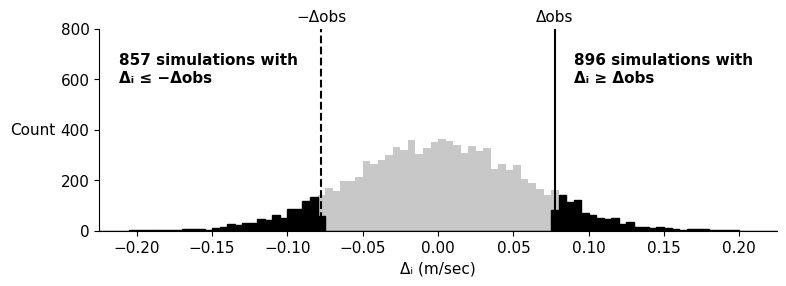
Figure 6.39 — Paired differences plot
fig, ax = plt.subplots(figsize=(5, 4.5))
for s, w in zip(swimsuit, wetsuit):
    ax.plot([0, 1], [s, w], 'k-', lw=0.8, zorder=2)
ax.scatter([0] * len(swimsuit), swimsuit, color=COLOR_SWIM, s=60, zorder=3)
ax.scatter([1] * len(wetsuit),  wetsuit,  color=COLOR_WET,  s=60, zorder=3)
ax.set_xticks([0, 1])
ax.set_xticklabels(['Swimsuit', 'Wetsuit'], fontweight='bold')
ax.set_ylim(1.08, 1.82)
ax.set_xlim(-0.3, 1.3)
ax.set_ylabel('Swimming speed\n(m/sec)', rotation=0, ha='center', va='center', labelpad=50)
despine(ax)
plt.tight_layout()
plt.show()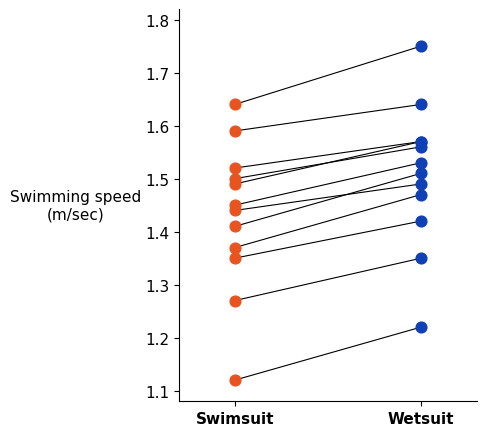
Figure 6.42 — Paired null distribution (sign-flip resampling)
fig, ax = plt.subplots(figsize=(8, 3))
ax.hist(ds_pair, bins=BINS, color='red')
ax.axvline(-dobs, color='black', lw=1.5, linestyle='--')
ax.axvline( dobs, color='black', lw=1.5, linestyle='-')
ax.text(-dobs, 1.02, '-Delta_obs', color='black', ha='center', va='bottom',
        transform=ax.get_xaxis_transform(), fontsize=11)
ax.text( dobs, 1.02, 'Delta_obs', color='black', ha='center', va='bottom',
        transform=ax.get_xaxis_transform(), fontsize=11)
ax.text(0.03, 0.88,
        f'{n_pair_lo} simulations with\nDelta_i <= -Delta_obs',
        transform=ax.transAxes, fontsize=11, fontweight='bold', va='top', ha='left')
ax.text(0.70, 0.88,
        f'{n_pair_hi} simulations with\nDelta_i >= Delta_obs',
        transform=ax.transAxes, fontsize=11, fontweight='bold', va='top', ha='left')
ax.set_xlabel('Delta_i (m/sec)')
ax.set_ylabel('Count', rotation=0, ha='center', va='center', labelpad=20)
ax.set_xlim(-0.225, 0.225)
despine(ax)
plt.tight_layout()
plt.show()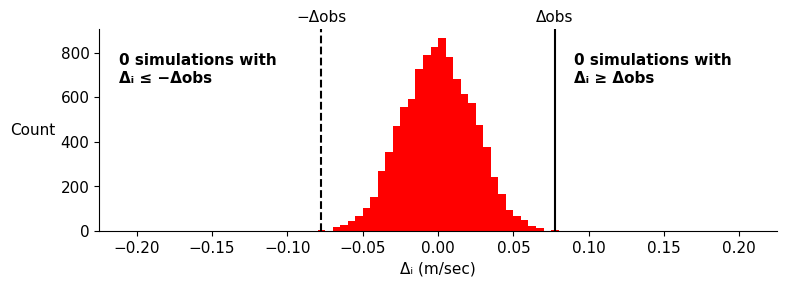
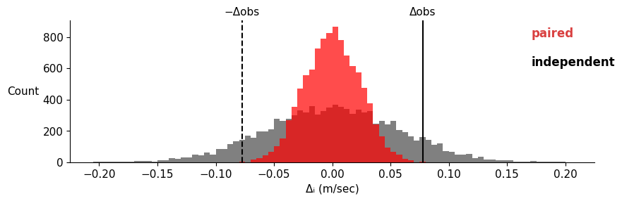
Figure 6.43 — Paired vs independent null distributions
fig, ax = plt.subplots(figsize=(9, 3))
ax.hist(ds_ind,  bins=BINS, color='gray')
ax.hist(ds_pair, bins=BINS, color='red', alpha=0.7)
ax.axvline(-dobs, color='black', lw=1.5, linestyle='--')
ax.axvline( dobs, color='black', lw=1.5, linestyle='-')
ax.text(-dobs, 1.02, '-Delta_obs', color='black', ha='center', va='bottom',
        transform=ax.get_xaxis_transform(), fontsize=11)
ax.text( dobs, 1.02, 'Delta_obs', color='black', ha='center', va='bottom',
        transform=ax.get_xaxis_transform(), fontsize=11)
ax.text(0.88, 0.95, 'paired',      color='#d94040', transform=ax.transAxes,
        fontsize=12, fontweight='bold', va='top', ha='left')
ax.text(0.88, 0.75, 'independent', color='black',   transform=ax.transAxes,
        fontsize=12, fontweight='bold', va='top', ha='left')
ax.set_xlabel('Delta_i (m/sec)')
ax.set_ylabel('Count', rotation=0, ha='center', va='center', labelpad=20)
ax.set_xlim(-0.225, 0.225)
despine(ax)
plt.tight_layout()
plt.show()